Lessons from convex optimization
In the last four weeks, I taught about convex optimization to my bioinformatics students. Since this topic is of general interest to those working with data and models, I will try to summarize the main points that the 'casual optimizer' should know. For a much more comprehensive overview, I refer to the excellent textbook of Boyd and Vandenberghe referenced below.
Convex functions
A convex set is a set for which every element on a line segment connecting two points is also in this set.
A convect function is a function for which the input domain is convex and for which it holds that
meaning that any line segment connecting two points on this curve lies above the curve.
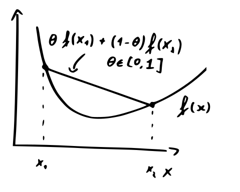
If the function is differentiable it also holds that the first-order Taylor approximation lies below the curve:
Convex functions are nice because when it has a minimum, this minimum is a global minimum. Such functions frequently arise in statistics and machine learning. Many machine learning methods, such as the support vector machine, are specifically posed as convex optimization problems.
Quadratic function
An important special case of convex functions are quadratic minimization problems:
with symmetric and positive-definite (i.e. all eigenvectors are greater than zero).
These have a closed-form solution:
Quadratic systems are important for least-squares-based learning and in certain graph problems. From a theoretical point of view, they are important because convex problems can be closely approximated by quadratic functions near their minimum, the region we are interested in!
General descent algorithms
For general convex optimization problems, one usually uses descent algorithms. The pseudocode of the general algorithm is given below.
given a starting point
repeat
Determine descent direction
Line search. Choose .
Update. .
until stopping criterion is reached.
Output:
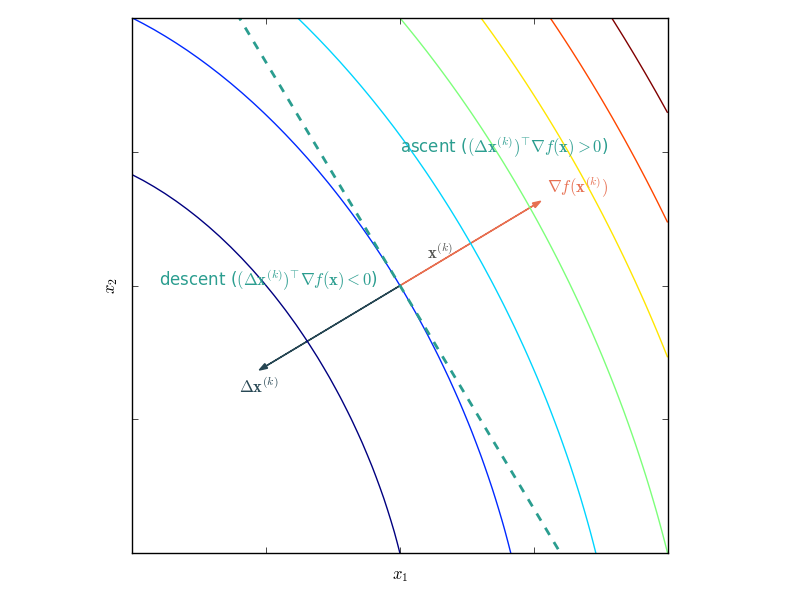
Descent algorithms differ by their descent direction, method for choosing the step size and the convergence criterion (often based on the norm of the gradient).
Proper descent methods have that
Gradient descent
A straightforward choice for the step size is the negative gradient:
Though this seems to make sense, in practice the convergence is rather poor. If is strongly convex (constants and exist such that ), it holds that after at most
iterations, where .
We conclude:
The number of steps needed for a given quality is proportional to the logarithm of the initial error.
To increase the accuracy with an order of magnitude, only a few more steps are needed.
Convergence is again determined by the condition number . Note that for large condition numbers: , so the number of required iterations increases linearly with increasing .
So the convergence is mainly determined by the shape of the function. See below for the example of the convergence on a quadratic and non-quadratic function.
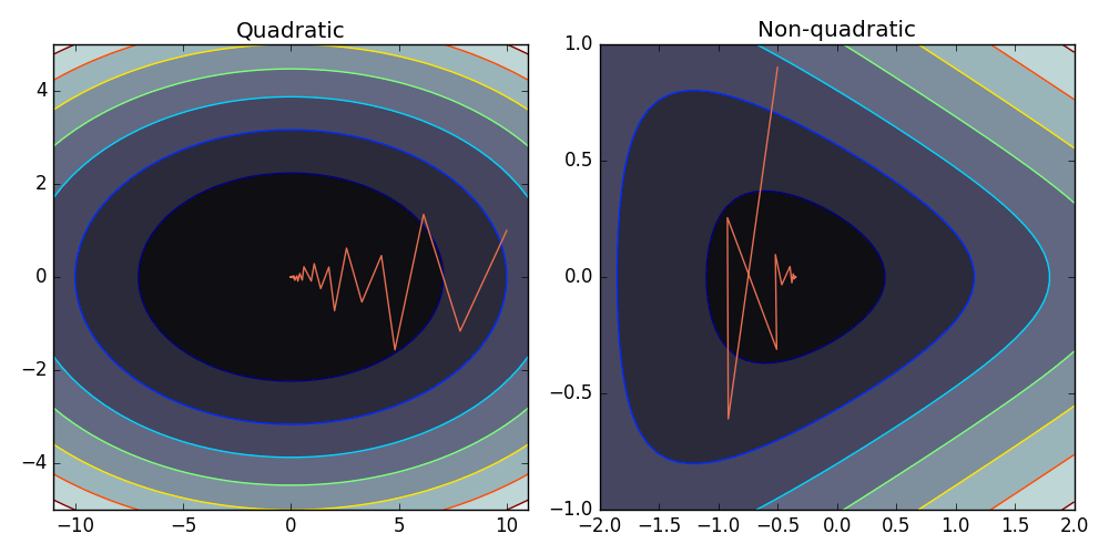
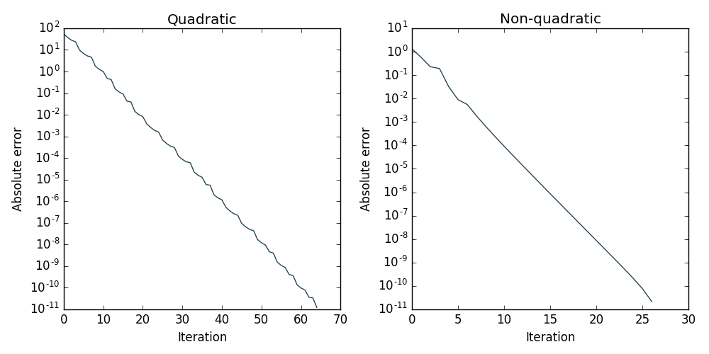
Note that even for such simple two-dimensional problems, pure gradient descent takes a long time to converge.
Newton's method
The main idea of Newton's method is approximating a function with a second-order Taylor approximation of at :
which is a convex quadratic function of . The Newton step is the step that minimizes this approximation in . The step is hence given by
Using the newton step in the general descent algorithm generally leads to a very fast convergence, especially when close to the minimum. Newton's method is much more robust to bad condition numbers and is affine invariant, scaling, translating or rotating the input domain does not influence its performance.
Linear equality constraints
Sometimes we want to minimize a function with respect to a linear equality constraint:
where is convex and twice continuously differentiable and with a rank .
A special Newton step which respects these constraints can be obtained by solving the following system:
Note that:
If the starting point is chosen such that , the residual term vanishes and steps will remain in the feasible region. This is the feasible start Newton method.
If we choose an arbitrary dom , not satisfying the constraints, this is the infeasible start Newton method. It will usually converge rapidly to the feasible region (check the final solution!).
Inequality constraints
Dealing with inequality constrains is more complex. In general, we want to solve
where are convex and twice continuously differentiable.
A trick is reformulating the problem using soft constraints in the objective function:
where we used the logarithmic barrier to approximate the inequality constraints. The parameter determines the sharpness of the approximation, as illustrated below.
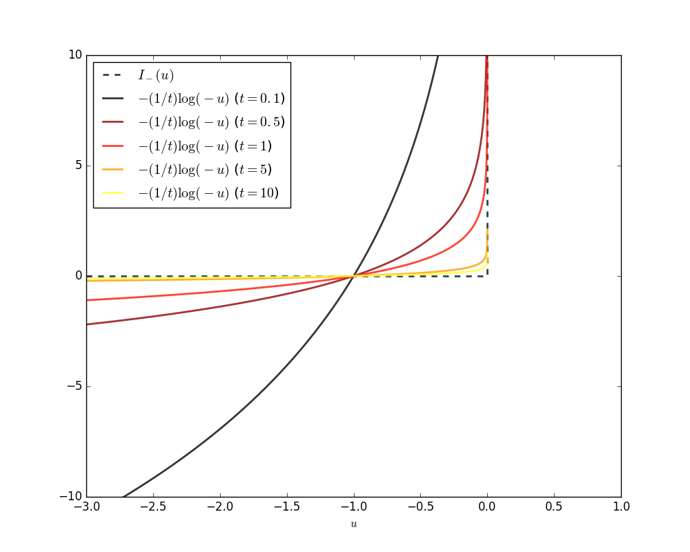
High values of result in a very good approximation but are hard to optimize because they are ill-conditioned. Interior point methods start with a low value of to obtain an initial solution and iteratively use the previous solution as a starting point for the soft-constrained optimization problem with increased .
References
Boyd, S. and Vandenberghe, L., 'Convex Optimization'. Cambridge University Press (2004)
Bishop, C., Pattern Recognition and Machine Learning. Springer (2006)